Fuzzy matching: comparison of 4 methods for making a join

In a previous article, I shared with you a solution to make a fuzzy matching between 2 different tables. I had then compared 2 ETL (Extract Transform Load) solutions. Tableau Prep Builder did not achieve the desired result. So, I turned to Anatella. In today’s article, I explore the different Fuzzy Matching algorithms available in this tool and their effects. As you will see, an algorithm emerges as the winner of the confrontation.

Introduction

When you want to make a join between several tables, you have 2 solutions. Either your join key follows precisely the same nomenclature in both tables, or it does not. If you’re in the blessed case of the first situation, please proceed, this article won’t teach you anything. If, on the other hand, you are in the 2nd case (or simply curious), I wish you happy reading.

Fuzzy matching algorithms

In the case study that I propose to you, the fuzzy matching is performed on a join key that contains country names. There are many methods for calculating the similarity between 2 entities. What I like about Anatella is that unlike other ETLs, it offers you a choice of 4 methods:

• Damereau Levenshtein distance
• Damereau Levenshtein similarity (the same as the distance even bounded between 0 and 1)
• Jaro Winkler similarity
• Dice similarity

There are, of course, other methods of calculating similarity. Raffael Vogler gives a good overview of the different techniques available in the “stringdist” package for R.

Jaro-Winkler similarity

The method dates from 1999 and is an evolution of Jaro’s method (1989). The score obtained varies between 0 and 1 and is calculated by comparing the corresponding characters in one string and then in the other, taking into account the character transpositions.

Damereau Levenshtein distance

The method is old (1964) and allows to calculate the number of steps needed to transform a string (a) into a string (b). Permitted operations are deletion, insertion, the substitution of a single character, transposition of 2 adjacent characters. The calculated distance is, therefore, a whole number that corresponds to the number of steps necessary for the transformation (0 when strings a and b are identical).

DICE similarity

The method is also long-standing (1948) and consists of a simple comparison of digrammes. The coefficient is close to Jaccard’s index. I direct you to Wikipedia for some telling examples.

The results

Here are the results. I would remind you that these are not transposable to any particular case. Each case must be studied beforehand to find the most suitable method. In this case, we are talking about fuzzy matching between country names that correspond to different nomenclatures. I refer you to my article from last week for the list of cases.

To compare the results produced by the different algorithms, I modified a little the flow in the ETL (Anatella) to put in parallel the 4 types of “fuzzy joins” proposed. The process is shown in blue on the diagram below (click on it to enlarge).

For ease of reading I have exported the results to an Excel file (download here).

The results are sometimes astonishing.

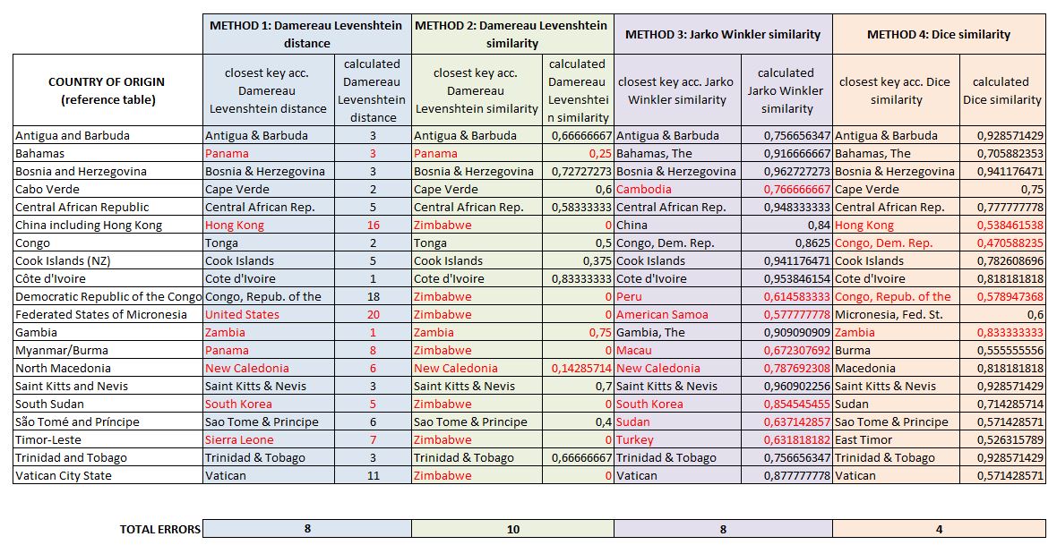
Method 2 seems to be the preferred method for Zimbabwe and differs from method 1 (which is more or less close). We can see that classification errors are sometimes quite crude (South Sudan / South Korea).

Method 3 (Jaro Winkler) is slightly better, but the classification errors are still too frequent. However, it has a significant advantage (see next paragraph).

Method 4 (Dice similarity) gives the best results. The misclassification of Hong Kong can be attributed to obvious reasons (see the entry in the reference table). The error on “Gambia” is easily explained by the digrammatic approach of the Dice-Sorensen method.

Definition of a threshold coefficient

To avoid ending up with false positives or false negatives, it is useful to define a threshold coefficient to reject results that require manual processing.

For Damereau Levenshtein’s method (methods 1 and 2) we see that this approach is not very efficient because the algorithm gives false positives with low calculated distances (see Bahamas, Gambia, North Macedonia, South Sudan).

For Dice, the definition of a threshold around 0.5 would not have made it possible to detect the 2 false positives and would also have delivered a false negative (Congo).

For Method 3, setting the threshold at 0.8 would have eliminated all missed matches but would also have generated a false negative (Trinidad and Tobago).

Conclusion

Dice’s method (also called Sorensen’s method) delivers in this exercise the best results to realise a fuzzy matching join between country names. The Jaro-Winkler method, on the other hand, makes it possible to define a threshold at 0.8, which precisely eliminates inconsistent results.

By Pierre-Nicolas Schwab Pierre-Nicolas est Docteur en Marketing et dirige l'agence d'études de marché IntoTheMinds. Ses domaines de prédilection sont le BigData l'e-commerce, le commerce de proximité, l'HoReCa et la logistique. Il est également chercheur en marketing à l'Université Libre de Bruxelles et sert de coach et formateur à plusieurs organisations et institutions publiques. Il peut être contacté par email, Linkedin ou par téléphone (+32 486 42 79 42)